Psychological Distress and Net Worth: An Econometric Investigation
This study applies OLS-based econometric and statistical modelling in SAS EM to reveal how psychological distress shapes wealth accumulation.
1. INTRODUCTION
Wealth accumulation and the factors that influence it are essential topics in socio-economic research. Net worth, defined as the sum of total assets minus total debts, is influenced by various factors, including the economic environment, policy changes, individual financial decisions, and demographic characteristics. However, an often overlooked aspect is the role of psychological factors, which can profoundly impact financial behaviour and outcomes.
This report examines the specific impact of psychological distress on net worth. For this purpose, the study is modelled using Ordinary Least Squares (OLS), which is analysed in the SAS EM using a simulated data set.
2. METHODOLOGY
In this study, ordinary least squares (OLS) regression analyses were used to investigate the effect of psychological distress (PD) on wealth.
2.1 Variables
(1)Explanatory Variables: PD (psychological distress), age, male, education, income, employed, socioeconomic status
(2)Response Variable: wealth
The variables ‘socioeconomic’ and ‘wealth’ were transformed using the ARSINH function. The transformed variables, ARSINH(socioeconomic) and ARSINH(wealth) were then used in the analysis.
2.2 Dummy Variable
Among the variables used in the model, ‘male’ and ‘employment’ are dummy variables.
In addition, to explore differences in economic behaviour across life stages, age was divided into three groups, represented by two dummy variables —— age25 and age65.
Table 1. Definitions for the dummy variables
| Variable Name | Description |
|---|---|
male | Equal to 1 if the respondent is male, and 0 otherwise |
employed | Equal to 1 if the respondent is employed, and 0 otherwise |
age25 | Equal to 1 if the respondent is younger than 25, and 0 otherwise |
age65 | Equal to 1 if the respondent is over 65, and 0 otherwise |
The ages are grouped according to the economic behaviour characteristics at different stages of life. After the age of 25, most people start their careers and begin to earn a substantial income, while after the age of 65, most people are likely to receive a pension when they retire.
2.3 Data preprocessing
After the data's initial exploration, extreme values in the 'wealth' and 'socio-economic' variables were removed. Both variables were then transformed using the ARSINH function. This transformation reduced the skewness of these variables and mitigated the extremity of their distributions.
2.4 Correlation Matrix Analysis
This analysis focuses on the impact of the variable pd on wealth. To achieve this, we have calculated Pearson's correlation coefficients, focusing on variables highly correlated with pd or wealth.
2.5 Manual Model Building and improving Models
2.5.1 Model 1 Impact of Income and PD on Wealth
The first model, starting with the effect of PD on WEALTH, gradually adds the variable INCOME to examine the effect of PD on WEALTH in depth. In total, three models were attempted:
Model 1.1
Model 1.2
Model 1.3
The final equation for the Model 1 was:
2.5.2 Model 2: Impact of Income Socioeconomic and PD on Wealth
In model2, socioeconomic variables were added to further explore the effect of the PD coefficients on wealth.
The equation for the Model 2 was:
2.5.3 Model 3: Impact of pd on wealth by gender
From the correlation matrix analysis, it was found that gender and pd were somewhat correlated. It was hypothesised that the magnitude of the effect of pd on wealth might be different for different genders, so in model 3, a male dummy variable and the interaction term pd*male were added.
The equation for the Model 3 was:
2.5.4 Model 4: Education’s Role in PD-Wealth Dynamics
In this section, the education variable was added to the model to further optimize it. Three models were attempted in total. Finally, after adjusting the interaction term from pd*education to pd*(education-13), the coefficients on the pd and pd quadratic term retained statistical significance.
The equation for the Model 4 was:
2.5.5 Model 5: Age Impact on PD-Wealth Relationship
It has been hypothesized that age is another factor influencing the extent to which pd explains wealth. Therefore, age was grouped by setting up a dummy variable to examine the effect of pd on wealth for people at different life stages.
By setting dummy variables, age is divided into under 25, 25-65 and over 65. This division is because individuals typically exhibit different economic behaviors at different stages of life; the period before the age of 25 is usually a period of learning and preparing for a career, while the age of 65 is a typical retirement age, marking the transition from full-time work to retirement.
Dummy variables are set as follows:
age25: Equal to 1 if the respondent is below age 25, and 0 otherwise.
age65: Equal to 1 if the respondent is above age 65, and 0 otherwise.
Also, the interacting items for dummy variables and pd were set up.
The equation for the Model 5 was:
2.5.6 Model 6&7: Sub-sample analysis of different wealth levels
To gain insight into how individuals differ according to wealth status, this study classifies observations into two categories according to wealth,
(1) Negative wealth group: a subset of 9,488 observations with wealth values less than zero.
(2) Positive wealth group: a subset of 55,778 observations with wealth values greater than zero and wealth values equal to zero.
The reason for this division is the assumption that the two populations' economic behavior may differ. After attempts and adjustments to the models, two separate models are finally obtained:
The equation for the Model 6(negative wealth group) was:
The equation for the Model 6(positive wealth group) was:
2.6 Classical Linear Regression Model (CLRM) Assumption Tests
The CLRM hypothesis test is applied to three different models:
Model 5: The final model for the full sample without grouping wealth values.
Model 6: The final model focusing on the negative wealth group,
Model 7: The final model focuses on the positive wealth group, including those observations with wealth values greater than or equal to zero.
2.6.1 The Average Value of Error Terms is Zero
To satisfy this assumption, the regression model must include an intercept.
2.6.2 Test for Heteroskedasticity
White's test is conducted to test for Heteroskedasticity.
2.6.3 Testing for Multicollinearity Among Independent Variables
The Variance Inflation Factor (VIF) is used to check for multicollinearity between variables in the model. A high VIF indicates that the variable is highly correlated with other independent variables.
2.6.4 Testing for Autocorrelation in the Residuals
The Breusch-Godfrey test was used to examine the autocorrelation of the residuals of the regression model.
2.6.5 Testing the Normality of Error Terms
The Jarque-Bera test was used to check the normality of residuals in regression models.
2.6.6 Test for model misspecification
Finally, Ramsey's RESET test was performed to see if the model was misspecified.
3. RESULTS AND DISCUSSION
3.1 General Descriptive Statistics and data preprocessing
3.1.1 General Descriptive Statistics
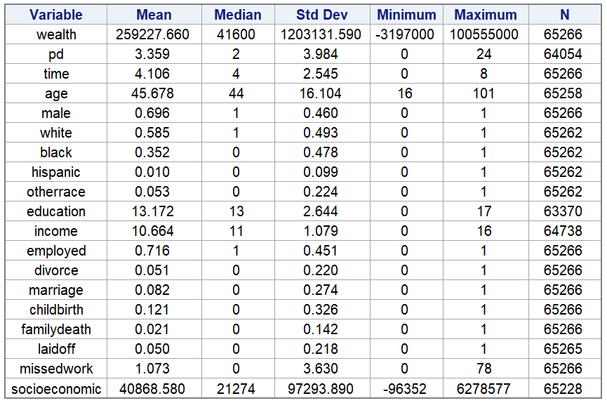
The table below shows the descriptive statistics of the original dataset.
There are about 65,000 observations in total. Most of the variables have the same or close number of observations, but Education and Income have slightly fewer observations, which could mean that there are missing values.
The mean of the Wealth variable is much higher than the median, suggesting that the data may be right-skewed and have extremely high values. This is also confirmed by the high standard deviation value, indicating significant wealth differences between individuals. The smallest value is negative, representing the presence of indebted people in the observed data. The Socioeconomic variables also exhibit a high degree of skewness and dispersion, with a median well below the mean, a significant standard deviation, and negative values in the data.
Male, White, Black, Hispanic, Other race, Employed, Divorce, Marriage, Childbirth, Family death, Laid off, and Missed work are dummy variables with values between 0 and 1.
Based on the mean value of the gender variable (Male), approximately 69.6% of the sample is male.
Among the race variables, White is the major group (about 58.5%) followed by Black (about 35.2%).
Variables representing major life events, such as Divorce, Marriage, Childbirth, Family death, Laid off, have means that represent the prevalence of the event, which can be seen from the means to indicate that these events do not occur in the majority of observations.
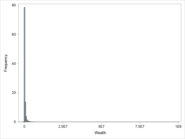
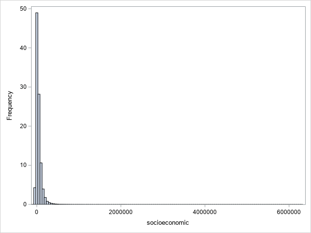
1.2 Histograms were plotted to confirm the data distribution for the wealth and socioeconomic variables further.
Both plots show the highly skewed distribution of the data. Most of the observations are clustered around the lower values, with some very high values, resulting in a long-tailed distribution. This suggests that a small number of people own most of the wealth. In this case, there may be extreme values.
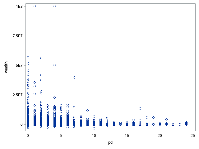
1.3 Outlier
After analysing the scatter plots for the wealth and socioeconomic variables, several extreme values were noted, which can be considered outliers. Considering that wealth is usually concentrated among a small number of people in a society, its distribution naturally exhibits a certain degree of skewness, and therefore, our model should reflect this social reality. However, to avoid the risk of those extreme outliers adversely affecting the model results, we removed the two largest values in the wealth variable and the three largest values in the socioeconomic variable. This strategy aims to remove those outliers with the most significant degree of deviation while retaining the characteristics of the skewed distribution in order to study the various effects in the context of this distribution.
The following figure shows a scatter plot comparison of these two variables before and after removing the outlier.
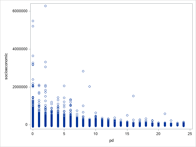
(A) Before removing outlier
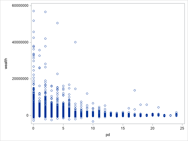
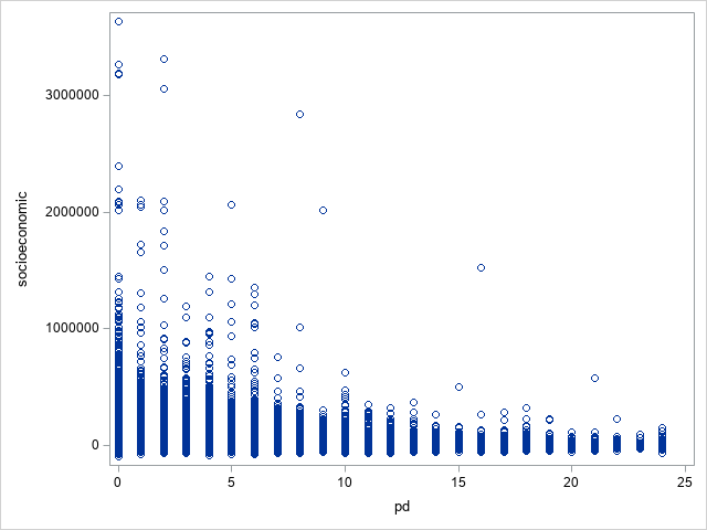
(B) After removing outlier
1.4 Data transformation
Because of the high skewness of the wealth and socioeconomic variables, these variables need to be log-transformed to better handle and interpret the data in subsequent analyses.
Due to negative values in the wealth and socioeconomic variables, the logarithmic transformation cannot be performed directly. Therefore, the arc hyperbolic sine transform will be used. This method facilitates the computation of logarithmic values of negative and positive numbers, thus making it suitable for zero and negative values in the dataset. In addition, it maintains the interpretability of the coefficients.
The following figures (A) and (B) show the data distribution after completing the arc hyperbolic sine transform.
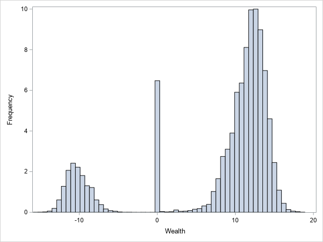
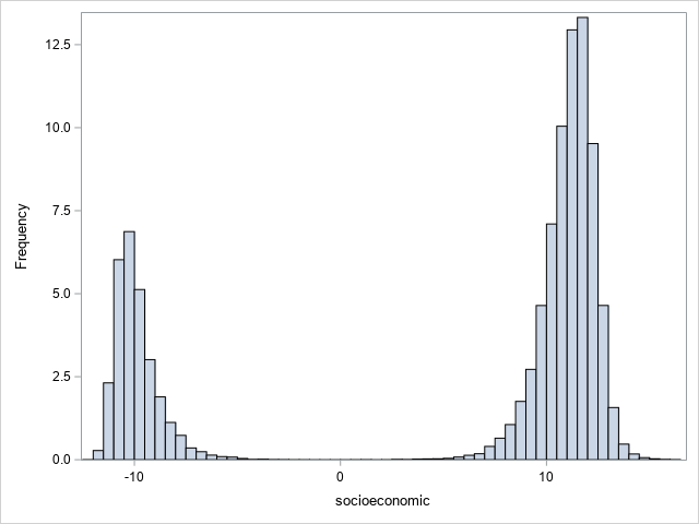
The distribution of the wealth variable shows a bimodal pattern on both sides, while some of the data are concentrated around the zero value, dividing the distribution into three parts. This pattern can be interpreted as three distinct groups in the population: a negative assets group, a positive assets group and a group with assets balanced around the zero value. The zero-value group may represent the group whose assets are at the break-even point.
Similarly, the distribution of the socioeconomic variable shows two peaks on either side of the zero point. This bimodal distribution suggests two sub-groups of socioeconomic status: a lower-status group and a higher-status group.
1.5 Correlation Matrix of Selected Variables
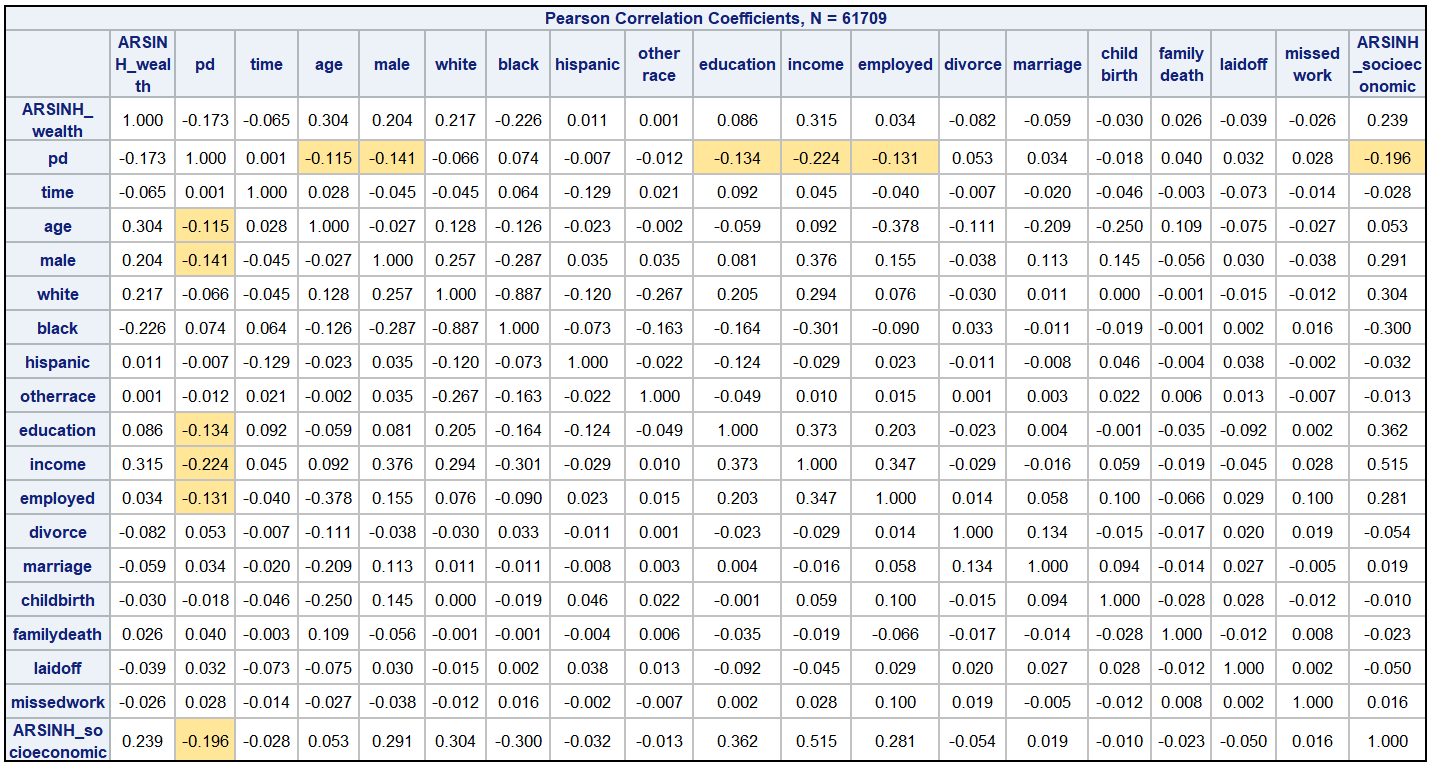
From the table above, pd is slightly correlated negatively with age(r=-0.115), suggesting that younger people may be more prone to higher levels of psychological distress. This may reflect the unique challenges and pressures faced by the younger population.
There is also a weak negative correlation(r=-0.141) between pd and male, which indicates a gender difference in the occurrence of psychological distress, suggesting that males have slightly lower levels of psychological distress than females in this sample.
The negative correlation(r=-0.134) between education and pd implies that those with higher levels of education may have slightly lower levels of psychological distress. This may be due to higher education improving problem-solving skills and resilience.
A moderate negative correlation(r=-0.224) between income and pd suggests that high levels of psychological distress may reduce earning capacity. On the other hand, it could also be the reason that financial security on mental health, with more financial resources buffering stress.
A slight negative correlation(r=-0.131) exists between employed and pd. Employment usually leads to a stable income and a sense of purpose, and therefore may help to reduce psychological stress.
A moderate negative correlation(r=-0.196) between pd and socioeconomic suggests that people of lower socio-economic status tend to experience higher levels of psychological distress. This may be because lower socio-economic status means limited access to economic resources and social support, which will result in some degree of psychological stress.
3. Results of the Model Building
3.1 Model 1: Impact of Income and PD on Wealth
3.1.1 In the initial model, only the effect of pd on wealth was examined.
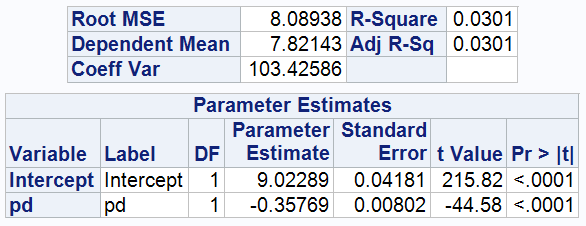
The model shows that the estimated value of the intercept is 9.02196, which can be interpreted as the baseline level of an individual's wealth status in the absence of psychological stress (pd=0). The coefficient of pd is -0.35762, indicating a negative correlation, meaning that the higher the psychological distress, the lower the level of wealth, specifically, for every unit increase in pd, the level of transformed wealth (ARSINH(wealth)) decreases by an average of 0.35762 units. The explanatory power of the model is relatively low, with an R-squared value of 0.0301, indicating that the pd variable explains only 3.01 per cent of the variation in wealth.
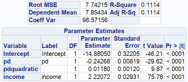
3.1.2
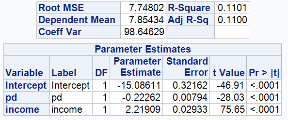
After the inclusion of the income, the intercept drops to -15.08611, indicating a lower baseline wealth level after accounting for the effects of psychological distress (pd) and income (INCOME). This may indicate that in the absence of psychological distress and income, individuals' wealth levels are at relatively low levels.
The coefficient of psychological distress (pd) also changes, reflecting the fact that the effect of pd on wealth may be overestimated without controlling for income. The addition of the income variable resulted in a coefficient of 2.21909 with a highly significant p-value (<0.0001), which implies that for every percentage point increase in income, ARSINH(WEALTH) is expected to increase by an average of 2.21909 units. This illustrates the important role of income in an individual's wealth level.
It can be inferred that an increase in psychological stress may lead to a decrease in the ability to generate income, which in turn affects an individual's wealth accumulation.
Finally, the R-squared value of the model has increased to 0.1100, which means that the new model explains changes in wealth levels better than the original model. Despite the improvement, the value is still relatively low, suggesting that the model does not explain most of the variation.
3.1.3 After finding that psychological distress (pd) has a negative effect on wealth, it was further hypothesised that the negative effect of pd on wealth may be exacerbated with increasing psychological distress.
The model was adjusted by adding a quadratic term for pd, which is pd*(pd-12). The [value of 12 is a threshold based on the Kessler Psychological Stress Scale (K6),]{.mark} whereby a score of more than 12 indicates the presence of a serious psychological problem.
The results of the model show that the coefficient of the quadratic term of psychological stress is 0.01180, which is positive, indicating that as psychological stress increases, its negative impact on the level of wealth gradually diminishes.
This may be due to the fact that individuals' ability to cope with high levels of psychological stress improves over time, thereby alleviating the negative impact on wealth.
Another speculation is that in real life, when psychological stress exceeds the threshold of 12, individuals may seek and receive more help from social support systems ( such as family, friends, and social service organisations), which can help to reduce some of the negative effects of stress on the economy.
After adjustments, The regression Model for Model 1 is:
3.2 Model 2: Impact of Income Socioeconomic and PD on Wealth
Model 2 focuses on the effect of the inclusion of the socioeconomic variable on the model.
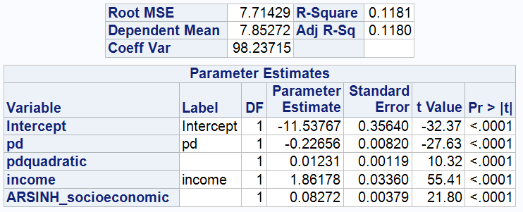
As can be seen from the table, the p-values for all parameter estimates are less than 0.0001, indicating statistical significance.
The coefficient of PD decreases from -0.24268 to -0.22656.Although this change is small, it suggests that socioeconomic status may influence the relationship between psychological distress and wealth to some extent. In other words, psychological distress in general has a negative effect on wealth accumulation, and there may be some subtle differences in this effect between high and low socioeconomic classes.
It can also be seen from the table that the income coefficient has decreased from 2.22072 to 1.86178. This suggests that the effect of income on wealth may be overestimated when socioeconomic is not included. This suggests that socioeconomic may include other wealth-related factors (for example, inheritance, investment income, etc.), especially in the higher socioeconomic status groups, which may be more important than wage income.
The coefficient for socio-economic status is 0.08272, which means that for every unit increase in ARSINH (socioeconomic), there is an increase of 0.08272 units in ARSINH (wealth). This positive coefficient also suggests that an increase in socioeconomic status provides individuals with more financial resources, better investment opportunities and more effective financial management services, all of which contribute to improved wealth accumulation.
The regression Model for Model 2 is:
3.3 Model 3: Impact of pd on wealth by gender
Model 3 incorporates the MALE variable to explore gender differences in the impact of pd on wealth.
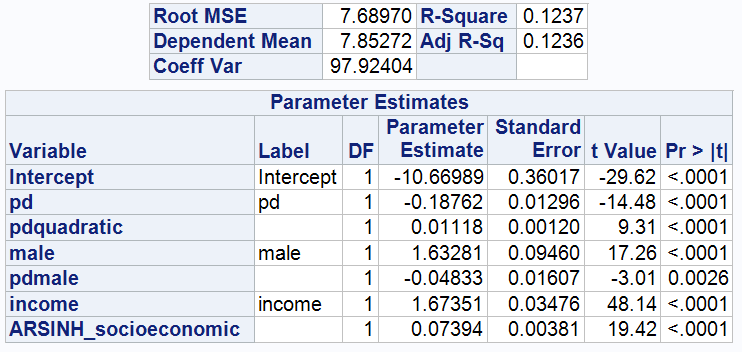
With the introduction of the new variable, the Adj R-sq for Model 3 improves from 0.1180 to 0.1236, and this slight improvement suggests that the model's ability to explain ARSINH(wealth) is not significantly enhanced.
The coefficients of both pd and pdquadratic change and the T-value decreases, indicating that the addition of the new variable calibrates the coefficients of pd but also increases the variability of the coefficients, making them more volatile.
The coefficient for male is 1.63281, indicating that men are on average 1.63281 ARSINH (wealth) units wealthier than women, holding all other variables constant.
In addition, an interaction term, pd*male, is introduced to examine the interaction between psychological stress and gender. The coefficient of this interaction term is -0.04833, indicating that as psychological stress increases, the wealth growth of males relative to females decreases. This implies that an increase in psychological stress has a more adverse effect on men's wealth than on women's wealth, thus reducing men's economic advantage.
This may be due to the fact that men may tend to take higher financial risks when making decisions, which normally benefits wealth accumulation. However, in high-stress situations, such risk-taking may lead to greater financial losses, thereby narrowing the wealth gap with women.
This may also be explained by the fact that women may exhibit greater mental and emotional resilience in the face of life's stresses. As stress increases, this resilience may help women to better manage stress and maintain job performance and income.
The regression Model for Model 3 is:
3.4. Model 4: Education's Role in PD-Wealth Dynamics
3.4.1 In this step, education variable is incorporated into the model.
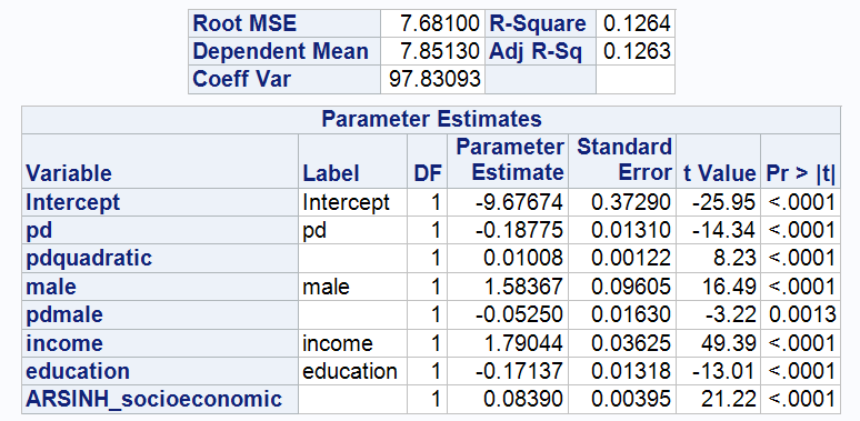
The table above shows that the coefficient on education is -0.17137, indicating that each additional year of education reduces ARSINH (wealth) by 0.17137 units on average. This suggests that higher levels of education are not directly associated with higher levels of wealth in the sample. This is somewhat counter-intuitive, as it is generally assumed that higher levels of education are associated with greater wealth, and this result may be influenced by other factors. For example, younger individuals may have just completed tertiary education and have not yet accumulated wealth, whereas older individuals with lower levels of education may have had more time to accumulate wealth.
In addition, the coefficients and T-values of pd and its quadratic term change very little after controlling for educational attainment, which provides a preliminary indication that the effect of pd on wealth may not be strongly related to educational attainment. In other words, excessive psychological stress appears to consistently reduce wealth regardless of educational level.
3.4.2 To investigate this hypothesis further, we introduced an interaction term between pd and education into the model.
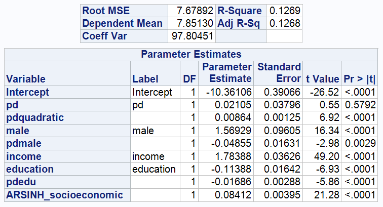
The table above shows that the p-value of the pd coefficient increases (p=0.5792) and the coefficient is no longer significant after adding pd*education. When this interaction term is added to the model, the pd coefficient now represents the effect of a one-unit change in pd on ARSINH (wealth) when education is zero. However, since most of the observations in the dataset do not have zero education, this may account for the reduced statistical significance of the pd coefficient.
3.4.3 It is also worth noting that the median and mean for education are both close to 13 years, which is roughly the time taken to complete secondary education. This suggests that the majority of people in society have completed at least secondary education, while only some choose to go on to higher levels of education. It is therefore appropriate to use 13 as a cut-off to adjust the interaction term to pd*(education-13). This adjustment sets the benchmark at the level of education at the end of high school and the beginning of college education, thus providing a more reasonable measure of how bias in years of education affects the impact of pd on wealth.
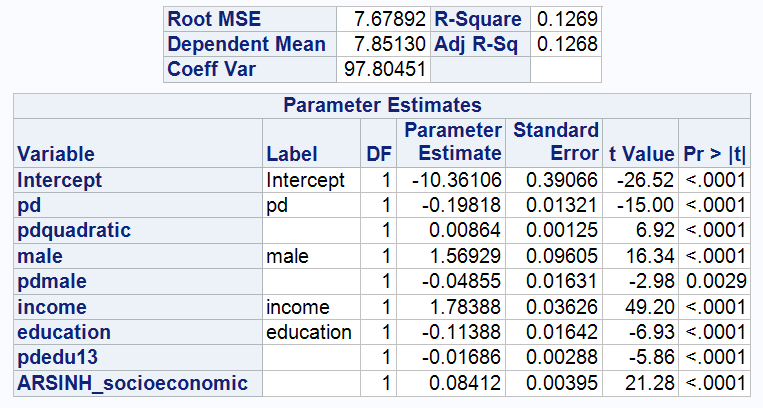
As can be seen in table above, the standard errors of pd and pdquadratic decrease and the t-values improve.
The pdedu13 coefficient is -0.01686, indicating that for individuals with more than 13 years of education, each additional year of education is associated with an additional increase in the negative impact of psychological distress, reducing ARSINH(wealth) by 0.01686 units, holding all else constant.
Specifically, if an individual is college educated or higher, they experience a greater decrease in wealth when dealing with psychological stress.
The reason behind this may be that higher education often comes with higher financial costs, such as student loans. These loans can put long-term financial strain on an individual. Additionally, while individuals with higher education may theoretically have more resources and skills to manage stress. However, they may also be exposed to more sources of stress, including work pressures, social competition, etc.
Another possible reason is that individuals with fewer years of education may have entered the labour market earlier, and the life and work experience they have gained may make them better able to cope with financial stress.
Finally, after adjustment, the model's Adjusted R-Sq improves very slightly from 0.1236 to 0.1268. this means that the current model can only explain about 12.68 per cent of the variance in ARSINH(wealth). While this change indicates an increase in the model's ability to explain variation, overall the adjusted coefficient of determination remains relatively low.
The regression Model for Model 4 is:
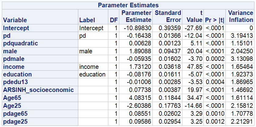
3.5 Model 5: Age Impact on PD-Wealth Relationship
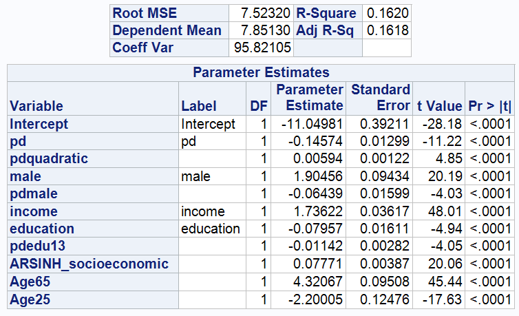
3.5.1 As can be seen in the table, holding all other variables constant, the coefficient of age65 compared to the benchmark group (age group 25-65) is 4.32067, meaning that people over 65 are on average 4.32067 ARSINH(wealth) units wealthier than the 25-65 age group, while people under 25 are 2.20005 ARSINH(wealth) units less wealthy than the benchmark group.
The t-value of PD drops from -15.00 to -11.22, indicating that the statistical significance of PD decreases with the inclusion of age, but the t-value is still much greater than 2, indicating that the effect of PD on wealth is still statistically significant even after controlling for age. This suggests that psychological stress is still an important factor influencing wealth.
Meanwhile, the coefficient of PD changed from -0.19818 to -0.14570, indicating that, controlling for age, the negative impact of psychological stress on wealth decreased. This may reflect the different ability to react and cope with psychological stress at different ages.
3.5.2 By incorporating the interaction terms pd*age65 and pd*age25, the effect of pd on wealth was examined for different age groups.
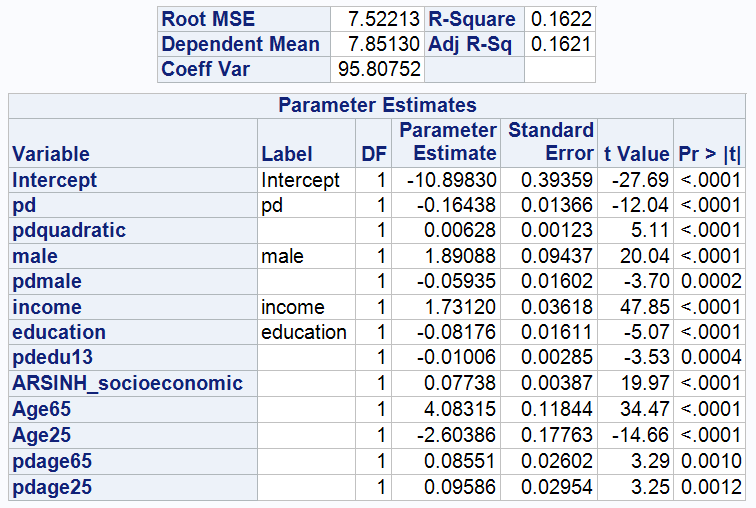
The coefficients on the interaction terms between pd and age group (over 65 and under 25) are both positive, 0.08551 and 0.09586 respectively, suggesting that psychological stress has a more positive impact on wealth in these age groups than in the middle-aged group (25-65), or that psychological stress has a less negative impact on their wealth accumulation.
This may be because people aged 25-65 tend to be under the double pressure of career development and family responsibilities and are often the main financial contributors to their families. Stresses such as job insecurity, divorce or parenting in this age group can directly reduce their wealth accumulation.
Young people under the age of 25 may adopt positive strategies to cope with stress, such as working overtime or taking on higher paid jobs, effectively turning stress into an incentive to accumulate wealth.
Also, most people over the age of 65 are likely to be retired and may have stable pensions and savings. Moreover, their rich life experience may provide them with more effective stress coping mechanisms.
The adj R-sq for this model improves to 0.1621, explaining 16.21% of the variance in the model.
The regression Model for Model 5 is:
3.6 Sub-sample analysis of different wealth levels
As this study focuses on the effect of PD on WEALTH, the main objective is to control for the statistical significance of PD while improving the unbiasedness of PD and the overall explanatory power of the model. There was also a focus on increasing the adj R-sq value to ensure that the explanatory power of the model was maximized. After fitting and optimization, two models were finalized:
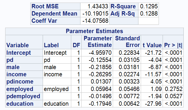
Model 6: Negative wealth Group
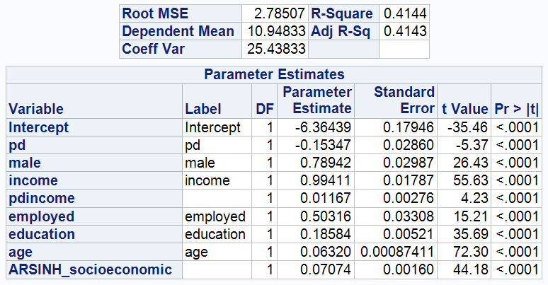
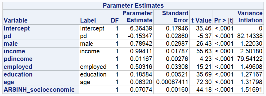
Model 7: Positive wealth Group
Comparing these two models and model 5, there are the following additional findings:
(1) The adjusted R-square of the Model 6 does not lift easily.
As can be seen from the two graphs above, Model 7 has an Adj R-sq of 0.4143, which is significantly higher than model 6 (Adj R-Sq: 0.1288) and model 5 (Adj R-Sq: 0.1621). Model 7 performs much better in explaining the variance in ARSINH(wealth). Specifically, Model 7 explains about 41.43% of the variation in the response variable ARSINH(wealth).
This difference may reflect the fact that the positive wealth group shows a more pronounced pattern and consistency in variables and wealth. In contrast, the negative wealth group lacks a clear pattern in these areas. This makes it more difficult to explain their wealth changes with a single model. There is also a possible reason for this: Model 6 does not include other important factors that have a significant impact on the financial situation, and these factors are not in the data set currently analysed.
(2)The coefficients of income are reversed in model 6 and model 7
The coefficients of INCOME for model6 and model7 are -0.26295 and 0.99411 respectively, which means that for the negative wealth group, ARSINH(wealth) decreases by an average of 0.26295 units for every 1% increase in income, holding all other variables constant and with a pd of zero. In contrast, for the positive wealth group, for every 1% increase in income, ARSINH(wealth) increases by an average of 0.99411 units, holding all other variables constant and with a pd of zero.
This means that for both groups, INCOME affects WEALTH in opposite directions. Typically, an increase in income leads to an increase in wealth. This is intuitive, since an increase in income provides more money for saving and investing, thus increasing an individual's total assets.
However, among the indebted, income is used more for consumption than for investment. This can affect wealth accumulation. In addition, an increase in income may also lead to an increase in consumption rather than debt repayment or savings. This phenomenon is often referred to as ‘lifestyle inflation’, in which individuals increase their standard of living and consumption habits as their income rises, possibly in the short term, without considering long-term financial security.
In addition, the interaction term Pd*income has a positive coefficient in both groups. This suggests that at higher incomes, psychological stress may act as an incentive to drive individuals to take action to maintain or increase their wealth, thus making it possible to get out of debt or accumulate assets more efficiently.
(3)The coefficients of male are reversed in model 6 and model 7
In Model 6, the coefficient of male is negative (-0.21856), indicating that men in the negative wealth group are on average 0.21856 ARSINH(wealth) units lower than women, controlling for other variables. In contrast, in Model 7, women in the positive wealth group are on average 0.78942 ARSINH(wealth) units lower than men.
This finding may imply that women are more cautious in accumulating wealth compared to men, preferring steady investment and long-term financial planning. This behaviour may have reduced the loss of their wealth during periods of economic instability, but it may also have limited the rate of wealth increase during periods of economic growth. Further analysis is needed to gain a deeper understanding of gender differences in wealth distribution and behaviour.
(4)Unlike Models 5 and 6, in Model 7, the coefficient on EDUCATION is positive
In Model 7, for the positive wealth group, the coefficient on education is positive (0.18584), indicating that for each additional year of education, an individual's ARSINH(wealth) increases by an average of 0.18584 units, controlling for other variables held constant. This suggests that in the positive wealth group, individuals with higher levels of education may already be earning a return on their investment in education.
2.8 CLRM Assumption Tests Results
2.8.1. The Average Value of Error Terms is Zero
Since the intercepts in Models 5, 6 and 7 all have p-values less than 0.0001, they are significant and must be included in the model. Keeping these intercepts ensures that the mean of the error term in the model is zero, which is consistent with the statistical assumptions of the CLRM.
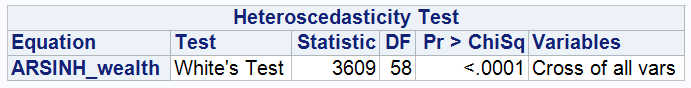
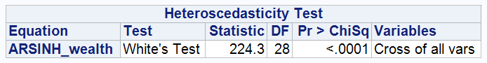
2.8.2 test for Heteroskedasticity
Model 5
Model 6
Model 7
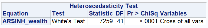
The p-values of White’s tests for Models 5, 6, and 7 were less than 0.0001. These results led to the rejection of the null hypothesis in White’s test, which posits that the disturbances are homoscedastic. Therefore, Models 5, 6, and 7 violate the assumption of homoscedasticity. The error terms in these models are heteroscedastic.
3. Testing for Multicollinearity Among Independent Variables
Model 5
As seen from the results, all of the variables have VIF values below 5, indicating low covariance between them.
Model 6
Model 7
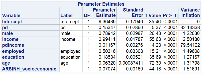
In Models 6 and 7, the VIF values for pd and its interaction term pd*income are significantly higher than the generally accepted thresholds, suggesting a high correlation between the two. This is consistent with our hypothesis that psychological distress (PD) may affect wealth accumulation through a direct correlation with income. This high degree of multicollinearity may affect the stability and reliability of the coefficients of these variables, as it may increase the standard errors of the coefficients and reduce the reliability of statistical tests.
4. Testing for Autocorrelation in the Residuals
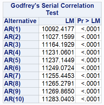
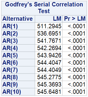
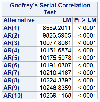
The table shows the results of the Breusch-Godfrey test for model 5, 6,
- The p-values corresponding to the Lagrangian multiplier (LM) statistics from the first order (AR(1)) to the tenth order (AR(10)) are extremely low (p<0.0001), providing sufficient evidence to reject the null hypothesis that the model residuals are not autocorrelated. That is, the error terms in Model 5, 6, 7 are correlated with each other.
The occurrence of this autocorrelation may be related to the fact that the dataset is panel data; the error of each observation at one point in time may affect its error at subsequent points in time. For example, the effect of individual psychological distress (PD) on wealth may carry over over time. Given this, the use of ordinary least squares (OLS) may not be the best way to analyse such data, as OLS assumes that the error terms are independent of each other, an assumption that may not hold for panel data.
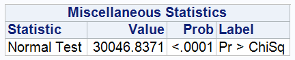
5. Testing the Normality of Error Terms
Model 5
Model 6
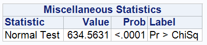
Model 7
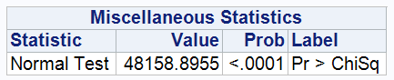
In Models 5, 6 and 7, the Jarque-Bera statistic is significantly high and the p-values are extremely low (p < 0.0001), indicating that the residuals in these models deviate from a normal distribution. Consequently, the null hypothesis that the residuals are normally distributed is rejected.
6.Test for model misspecification
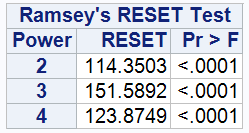
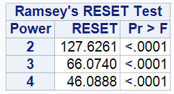
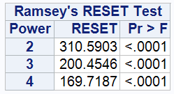
The results of the RESET test show that all p-values are well below the critical value of 0.0001, whether the test is performed on the second, third or fourth power of ARSINH(wealth). This provides strong evidence to reject the null hypothesis H0: the functional form of the model is correct, suggesting that existing models may not accurately capture the true relationship between explanatory and response variables. It could also mean that some important variables are missing from the model.
One possible explanation is a dynamic relationship that is not captured by the model. For example, the effect of an individual's psychological distress (PD) on wealth (Wealth) may not be immediately apparent, but may manifest itself over time, with a lag during which individuals may adjust their financial behavior.
Similarly, the positive impact of education on income is usually a cumulative process as individuals complete their education, enter the labor market and gain experience. In addition, given that the data span covers the period from 2003 to 2019, the model may fail to control for the impact of macroeconomic factors such as economic cycles and policy changes. Over such a long time span, global economic events or national economic changes may have had a significant impact on the wealth of individuals, all of which may lead to model misspecification if these factors are not properly accounted for and controlled for in the model.
4. CONCLUSION
This report examines the relationship between psychological distress and wealth accumulation, providing insights into the various factors that influence wealth through several models. The results suggest that psychological distress has a consistently negative effect on wealth, and this effect varies across populations.
The main findings of our modelling are that income and socio-economic status significantly buffer the negative effects of psychological distress. In addition, the impact of psychological distress on wealth varies by gender and age. Men and those in the 25-65 age group appear to have a greater negative impact on their wealth due to psychological distress, which may be due to their primary role in finances and the associated stress. Furthermore, the pattern of wealth accumulation is clearer for the positive wealth group than for the negative wealth group. For example, wealth is strongly influenced by variables such as education and employment, suggesting that the pathways of wealth accumulation are more predictable for those who already have wealth.
However, this study also finds some counterintuitive results, such as the fact that an increase in education levels seems to be associated with a decrease in wealth accumulation. This counterintuitive phenomenon may be due to the time-lagged effect of education on wealth. Typically, higher investments in education take years of work experience to pay off, and higher education loans may first have to be repaid. However, ordinary least squares (OLS) models may not be effective in capturing this dynamic time effect.
In addition, it is worth noting that the panel data used in this study has the characteristics of both time series and cross-sectional data. The OLS model assumes that the data are independent of each other, which may not be applicable to the characteristics of the panel data. The test results of the CLRM also indicate that the model may suffer from heteroskedasticity, autocorrelation and misspecification, which further suggests that the use of the OLS approach may not be appropriate.
Therefore, to better explore the impact of psychological stress on wealth accumulation, future research should consider modelling approaches that are more suitable for dealing with panel data, such as fixed or random effects models, which can better take into account the effect of time factors on variables.