Machine Learning Models for Image Recognition

Executive summary

This study aimed to achieve classification predictions for 19 specified celebrities using input image data.

The dataset used in this study contains 3334 celebrity image entries, each containing 10000 feature values. The initial data preprocessing stage involved reshaping row data into NumPy arrays of shape (100,100, 1) for single-channel grayscale images or (100, 100, 3) for RGB images. This preprocessed data was then fed into various training models. In addition, the labels in the dataset were encoded to facilitate the machine-learning process.

The dataset was divided into a training set (70%), a validation set (20%) and a test set (10%). Three models were trained during the study: ANN, OpenCV and CNN. The key performance metrics considered include precision, recall, F1 score and accuracy. The performance of each model was further analyzed through a confusion matrix to check for misclassification.

The CNN model demonstrated the best overall performance, with 81% precision, 78% recall, 78% F1 score, and 78% accuracy. Compared to the other models in the test, CNN is clearly more effective for image recognition tasks.

This study used Python, which was selected for its extensive and powerful libraries. These include NumPy for data manipulation, OpenCV for image processing, and various machine learning libraries such as TensorFlow and scikit-learn for model training and evaluation.

1.Introduction

This project aims to perform celebrity classification predictions using provided image data. The dataset comprises 19 predefined celebrity categories, and the objective is to classify inputs into these categories. Fundamentally, this research focuses on facial feature extraction and recognition classification, a field with significant implications across various domains.

The ability to accurately classify individuals in images has a wide range of applications, from security systems and personal identity verification to digital entertainment. By advancing our understanding and capabilities in facial recognition, we can develop more sophisticated and reliable systems that can be deployed in real-world scenarios.

Facial recognition techniques have evolved significantly over the years. Initially, systems such as Eigenfaces, developed in the 1990s, used linear algebra and principal component analysis to extract facial features. Over time, more advanced methods such as Fisherfaces and local binary patterns have been developed to increase the system's robustness. These methods recognize faces more efficiently under a variety of conditions.

The advent of deep learning has completely revolutionized the classification, identification, and facial recognition fields. Convolutional neural network (CNN) is a type of deep neural network that is particularly well-suited to image processing tasks. In contrast to traditional algorithms, which require manual feature extraction, CNN learns patterns directly from image pixels. Each layer of the network learns to recognize increasingly complex features.

Artificial neural networks (ANN) represent another foundational technology in facial recognition. While less specialized than CNN in dealing with spatial hierarchies, ANN is also crucial for tasks that require modelling complex non-linear relationships. As a result, it typically requires manual feature engineering to identify relevant facial features prior to training, which makes them less efficient than CNN in processing raw image data.

OpenCV, which stands for Open-Source Computer Vision, offers a comprehensive suite of tools for facial recognition. It includes methods such as Haar Cascades(Kaur & Mirza, 2021) and Histogram of Oriented Gradients (HOG), which were previously widely used before the advent of deep learning. 

This project will investigate the performance of CNN, ANN, and OpenCV in face recognition classification tasks. By in-depth investigation of these methods, we aim to accurately classify input information into the predefined 19 celebrity categories and uncover some insights into image recognition classification algorithms.

2.Materials and Methodologies

2.1 Materials

2.1.1 Dataset Description

2.1.1.1 Image files

The image files comprise 19 folders, each representing a different celebrity. Each folder contains approximately 200 or more facial images. The images include a variety of angles and expressions, with some individuals in the images wearing glasses or make-up, and some in black and white. The image size is not standardized, ranging from 100 to 500 pixels in width or length. 

The Table1 below provides an overview of information about the image files.

Table 1: Image statistics

Folder Name	Image Count	Min Resolution	Max Resolution
Alexandra Daddario	215	95×108	564×668
Amber Heard	208	102×105	550×668
Andy Samberg	186	95×108	550×658
Anne Hathaway	193	102×108	527×558
Chris Hemsworth	149	102×108	564×668
Chris Pratt	166	100×108	564×671
Dwayne Johnson	131	102×108	564×668
Emma Stone	129	102×108	527×558
Emma Watson	201	101×128	527×558
Henry Cavil	185	102×108	564×668
Hugh Jackman	169	99×108	527×558
Jason Momoa	174	102×108	564×802
Margot Robbie	211	102×108	564×802
Robert Downey Jr	223	93×108	558×668
Scarlett Johansson	191	102×108	564×668
Taylor Swift	121	102×108	489×547
Tom Holland	179	99×108	527×558
Zendaya	128	102×108	489×554
Zoe Saldana	176	102×105	527×554

2.1.1.2 Image data

The original dataset also contains image data in six spreadsheets, divided into two main categories: labelled and unlabelled datasets. Each category contains three image resolutions: 20*20, 50*50, and 100*100.

Table 2 below provides an overview of the image dataset.

Table 2: Image data statistics

Type	File Name	Number of Images	Features per Image
labelled	training_celeb20x20	3335	400
	training_celeb50x50	3335	2500
	training_celeb100x100	3335	10000
unlabelled	unlabelledtest_celeb20x20	3335	400
	unlabelledtest_celeb50x50	3335	2500
	unlabelledtest_celeb100x100	3335	10000

2.1.1.3 Selected dataset for analysis

In this study, we trained the model on labelled datasets, initially experimenting with image resolutions of 20x20, 50x50 and 100x100 to test the models. Finally, we decided to train three different models using the 100x100 resolution. We selected this resolution because it provides more detailed information than 20x20 and 50x50, which is crucial for the models to learn more complex features.

Specifically, we selected the following datasets for analysis:

• Labelled 100x100 dataset: Used to train the model.

• Unlabelled 100x100 dataset: Used to test the final results after the final deployment of the model.

1. Variable Description

The 100*100 labelled data set comprises two types of variables. The first column, 'celeb', represents the label, indicating the celebrity's name corresponding to each row of data. The data is of a string data type. The columns from the 2nd to 10001st represent the features of each image, with a float data type ranging from -1 to 1. The column names range from c1r1 (representing the features in the first row of the first column of the image) to c100r100.

In the unlabelled 100x100 dataset, the columns from the 1st to the 10000th are all feature variables, and there is no 'celeb' variable.

2.2 Methodologies

2.2.1 Data Preprocessing

2.2.1.1 A data integrity check was conducted on the dataset to identify any missing values, outliers, or duplicates. One duplicate row was then deleted. The distribution of data for each celebrity was then analyzed.

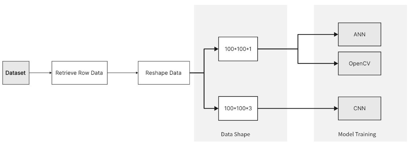
2.2.1.2 Reshape data As shown in figure 1, each row of data extracted from the dataset is converted into two shapes. The first shape is 100x100x1, representing a single-channel grayscale image used in ANN and OpenCV models. The second shape is 100x100x3, representing an RGB image used in CNN models. This format is ideal for deep learning models, especially convolutional neural networks, as it allows them to handle images with color information and complex features. The data reshaping is to meet the input requirements of different models, thereby enabling them to process and analyze the image data more effectively.

Figure 1: Data reshaping process

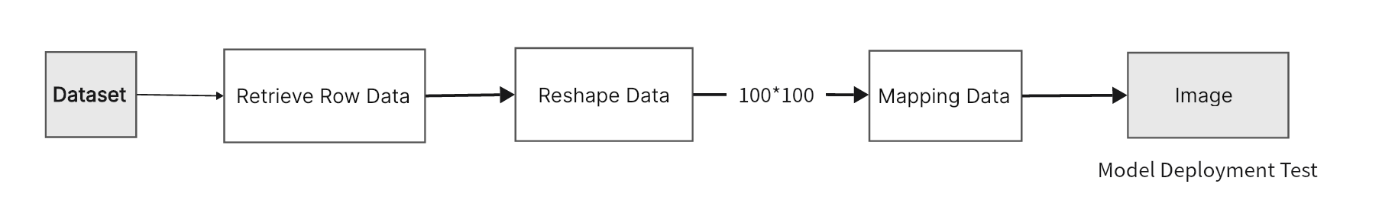
2.2.1.3 Mapping data

During the model deployment and testing process, the unlabeled dataset is mapped into actual image formats. The predicted name results from the model are then displayed directly above the images. This process helps visually verify the model's predictions.

Figure 2 shows that the row data is initially reshaped into a 100x100 NumPy array, which is then converted into an image.

Figure 2: Data mapping process

2.2.1.4 Encoding

The original labels in the dataset are of the string type and must be converted into formats suitable for machine learning models. 

We utilize the Sparse label encoding method. In this method, category labels are represented directly as integers. This approach is highly effective for handling large datasets.

2.2.2 Data Split

The 100 x 100 unlabelled dataset was divided into the following proportions:

(1) Training set (70%): used for the model training process and contains most data to ensure the model has sufficient learning information.

(2) Validation set (20%): used for performance validation during the model training process to avoid overfitting.

(3) Test set (10%): used to evaluate the final performance of the model after model training is complete.

2.2.3 Algorithm Description

2.2.3.1 Artificial Neural Network (ANN)

Artificial Neural Network (ANN) is a computing system. It consists of interconnected units or nodes that simulate the human brain's ability to recognize complex patterns and relationships in data. They are therefore often used for classification tasks.

Figure 3: ANN Model Architecture

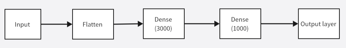
Figure 3 illustrates the architecture of the ANN employed in this project:

The input layer: It receives the reshaped image data and prepares it for processing.

The Flatten Layer: This process transforms the multi-dimensional image data into a one-dimensional array, enabling the extraction of features more efficiently.

Dense layers:

The initial dense layer comprises 3,000 neurons, which are essential for the learning of high-level features.

The second dense layer of 1,000 neurons serves to refine these features further.

The output layer: The trained features are then used to classify images by celebrity, resulting in the final predictive output.

2.2.3.2 Open-source computer vision library (OpenCV)

OpenCV is an open-source computer vision and machine learning software library. It offers a comprehensive range of image processing and recognition algorithms, which are well-suited to complex facial recognition tasks.

This study uses OpenCV's Local Binary Patterns Histograms (LBPH) algorithm for face recognition tasks. LBPH is a face-recognition algorithm used in image processing to identify faces by analyzing simple patterns within the image.

In this project, the LBPH face recognizer is first initialized. The recognizer is then trained using a training dataset of labelled face images. This phase involves learning the distinctive features of each face that are essential for distinguishing between different individuals.

2.2.3.3 Convolutional Neural Networks（CNN）

CNN is a deep learning method. By employing convolutional, pooling and fully connected layers, CNN can automatically learn and extract meaningful features from images. It is a highly effective tool for a range of image-related tasks, including classification, object detection and segmentation.

Figure 4: ANN Model Architecture and Optimizer Process

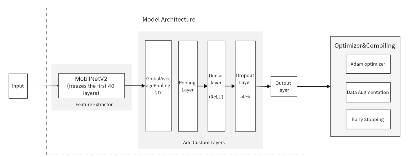
After a series of adjustments and optimizations, we selected a specific CNN model, as shown in Figure 4. This model's design is centered around two key components: the model architecture and model optimization.

(1) Model architecture 

The model architecture was developed using MobileNetV2 as the foundational structure, incorporating additional custom layers to enhance performance.

a) MobileNetV2

MobileNetV2 is a convolutional neural network architecture designed for mobile devices. It focuses on efficiency and effectiveness in feature extraction.

In this project, MobileNetV2 was selected as the feature extractor. The input shape was adjusted to three channels:100x100x3. This adjustment aims to leverage MobileNetV2's feature extraction capabilities to their full potential.

Furthermore, freezing layers represents a crucial strategy in the model. The initial 40 layers of the model are frozen to ensure the preservation of the base features learned by MobileNetV2. This operation guarantees that these base features will not be altered by the training process of the new dataset, enhancing the stability and training efficiency of the model.

b) Adding custom layers

Following the implementation of MobileNetV2, several custom layers were added to enhance the model's ability to handle specific tasks.

GlobalAveragePooling2D: Used to reduce the number of parameters, simplify the model and reduce the risk of overfitting.

Dense layer: Contains 128 neurons activated using ReLU, which introduces non-linearity to help the model learn complex patterns.

Dropout Layer: 50% of neurons are randomly discarded during training to prevent overfitting.

Output layer: Fully connected layer using a softmax activation function, which transforms the input into a probability distribution and calculates the probability of each celebrity category.

(2) Model Training Optimization

In the compiling and fitting session of the CNN model, we used some optimization strategies to improve the performance of the model:

a) Adam Optimizer: An iterative optimization algorithm designed for training deep learning models. It utilizes an adaptive learning rate mechanism to converge to optimal solutions efficiently.

b) Data Augmentation: The method artificially expands the training set by creating modified versions of the images in it. Our study augmented the facial dataset with various transformations, including rotation, scaling, stretching, and brightness adjustment. These modifications help to simulate different viewing conditions, providing a more diverse training dataset.

c) Early stopping: Monitors the model's performance on the validation set and stops training if the performance does not improve after several epochs. This prevents overfitting of the training data and saves time and computational resources.

2.2.4 Evaluation metrics

2.2.4.1 Precision

Precision measures the proportion of correct predictions for a given class out of all predictions made. High image classification precision means fewer non-target objects are mistakenly identified as the target class.

2.2.4.2 Recall

Recall measures the proportion of actual positives identified correctly by the model out of all actual positives. In this project, a higher recall indicates that the model effectively captures a larger portion of actual celebrity images.

2.2.4.3 F1 score

The F1 score provides a balanced measure of the model's accuracy and recall. In this project, a high F1 score indicates robust and balanced performance in identifying celebrity images precisely and comprehensively.

The formula for the F1 score is: $F1 = 2*(\frac{Precision \times Recall}{Precision + Recall}$)

2.2.4.4 Accuracy rate

Accuracy is the ratio of correct predictions to the total number of predictions made. In a project identifying 19 celebrities, a high accuracy rate means that the model effectively distinguishes and recognizes different celebrity faces.

2.2.4.5 Confusion matrix

The confusion matrix is a table that shows the number of correct and incorrect predictions by each category.

To evaluate our model's performance across the 19 celebrity categories, we used a confusion matrix to represent the accuracy of the predictions. The diagonal items of the matrix represent the correct classification of each category, while the off-diagonal items indicate prediction errors, indicating the number of times the model incorrectly labelled a category as another.

2.2.4.6 Training and validation accuracy curves

The training and validation accuracy curves demonstrate the model's effectiveness in predicting the target variable on the training and validation datasets over the epochs. This comparison helps assess the model's performance and its ability to generalize to unseen data.

3.Result

3.1 Data Preprocessing

3.1.1 Data clean

Figure 5: Distribution of Data per Celebrity

Figure 5 illustrates the quantity of image data for each celebrity, demonstrating variations between them. Robert Downey Jr. and Alexandra Daddario have the most significant number of images, with approximately 220 images each. Conversely, Taylor Swift, Emma Stone, Zendaya, and Dwayne Johnson have the lowest data volumes, with approximately 120 images each. The discrepancy in data volume between the highest and lowest categories is almost twice as significant.

The discrepancy in the data volume may bias our model, which could affect its performance in categories with less data. This issue may indicate a challenge in model training.

3.1.2 Reshaping data

To meet the input requirements of the model, we reshaped each row of data in the table dataset to 100x100x1, meaning that each piece of image data was processed as a single-channel (greyscale) image of 100x100 pixels. After processing, we took the first data of each celebrity in the table data and did the image mapping to preview it. By visualizing the data matrix, we confirmed that the conversion was successful.

Figure 6: Preview of reshaping data after converting to image

3.2 Model result

3.2.1 ANN

After training the ANN model, it was tested on the test set, achieving a final accuracy of 29%.

3.2.1.1 Precision, recall, F1-score

Figure 6 illustrates the precision, recall, and F1-score for each celebrity category using the ANN model.

Figure 7: The precision, recall and F1-score of ANN model

The figure illustrates a considerable variation in recall and precision among celebrities. Taylor Swift has a higher recall rate than the average celebrity but a lower precision rate. This indicates that while the model can identify most images of Taylor Swift, it also incorrectly classifies other celebrities as her, resulting in a higher number of false positives. This may be due to the learning of over-generalized features for this category. These features lack sufficient distinction to differentiate accurately between individuals with similar appearances.

On the other hand, celebrities such as Amber Heard, Emma Stone, Anne Hathaway, Jason Momoa, and Tom Holland showed high precision but low recall, suggesting that the model was more conservative in predicting these categories conservatively, missing many true positives. This may mean that the model is too strict in identifying these categories.

Margot Robbie has the highest F1 score, indicating that the model achieves a good balance between precision and recall for this celebrity.

3.2.1.2 Confusion matrix

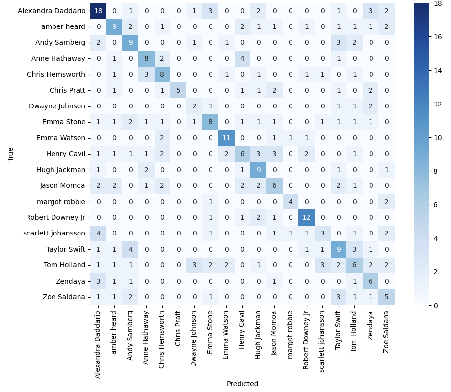
Figure 8: The confusion matrix of ANN model

Further analysis of the confusion matrix revealed that many of the celebrity images were misidentified as Taylor Swift and Alexandra Daddario. This suggests that the features learnt by the model from these two individuals may be too dominant or generic. This causes the model to be prone to misclassification when confronted with other celebrities with similar features.

On the diagonal, Emma Stone had the lowest value of 1, meaning that the model had great difficulty correctly recognizing images of her. This low accuracy suggests that the model may not be capturing the unique features needed to distinguish her accurately or that there is insufficient training data for this category.

3.2.1.3 Training, validation, and test accuracy

Figure 9: Training, Validation, and Test Accuracy (ANN)

As illustrated in Figure 9, the significant gap between the training and validation accuracy levels indicates overfitting. While the model performs well on the training data, it struggles to generalize to the validation data.

Furthermore, the relatively low and fluctuating validation accuracy and the stable but low test accuracy suggest that the model is not generalizing well to new data. 

3.2.2 OpenCV

After testing the OpenCV model on a test set, it achieved a final accuracy of 43%.

3.2.2.1 Precision, recall, F1-score

Figure 10: The precision, recall and F1-score of OpenCV model

As can be seen from the figure 10, there is not a large difference between precision and recall for most celebrities, which suggests that the model performs relatively evenly across the different celebrity categories.

However, Chris Pratt precision is much larger than the recall, this suggests that the model is usually accurate when predicting as Chris Pratt but misses many true cases.

Looking at the F1 scores, there is not much variation in values across celebrities, with the highest being Emma Watson, Margot Robbie, and Robert Downey Jr, suggesting that the categories of these celebrities achieve a better balance between precision and recall.

3.2.2.2 Confusion matrix

Figure 11: The confusion matrix of OpenCV model

Further analysis of the confusion matrix indicates that Alexandra Daddario, Robert Downey Jr. and Emma Watson have the highest values on the diagonal, suggesting that the model can recognize these celebrities with high accuracy. Conversely, Dwayne Johnson has the lowest value on the diagonal, indicating that the model has difficulty accurately recognizing him. This may be due to the model capturing fewer features or the training data being under-representative.

Tom Hollander and Emma Stone were frequently misidentified as other celebrities in the non-diagonal region, with a relatively even distribution across categories. This indicates that the model cannot distinguish between their features and those of other celebrities. This may be due to the model failing to capture their distinctive features effectively.

OpenCV shows lower false recognition values in the confusion matrix's non-diagonal region than in the ANN model. This suggests that the OpenCV model may have better feature discrimination ability when dealing with the face recognition task. In contrast, ANN may have some limitations in feature extraction and classification of categories, resulting in higher false recognition rates between certain celebrities.

3.2.2.3 Training, validation, and test accuracy

In OpenCV, the LBPH FaceRecognizer does not involve an iterative training process over multiple epochs. As a result, it is impossible to record training and validation accuracy for each epoch. Consequently, there is no concept of plotting training, validation, and test accuracy graphs for the OpenCV model.

3.2.3 CNN

3.2.3.1 Precision, recall, F1-score

The third method is based on CNN. The initial CNN model achieved an accuracy of 47%, higher than the ANN and OpenCV-based models. Building on this initial success, we optimized the CNN model further. The accuracy of our CNN model improved significantly, reaching approximately 78%.

Figure 12: The precision, recall and F1-score of CNN model

The figure 12 illustrates that the differences between precision and recall are relatively insignificant for most celebrities. In summary, all three metrics – precision, recall and F1-score – demonstrate superior performance compared to the ANN and OpenCV models.

These results also show that Emma Stone's recall and precision are below average, with recall being particularly poor. This indicates that the model has significant difficulty correctly recognizing images of Emma Stone. 

3.2.3.2 Confusion matrix

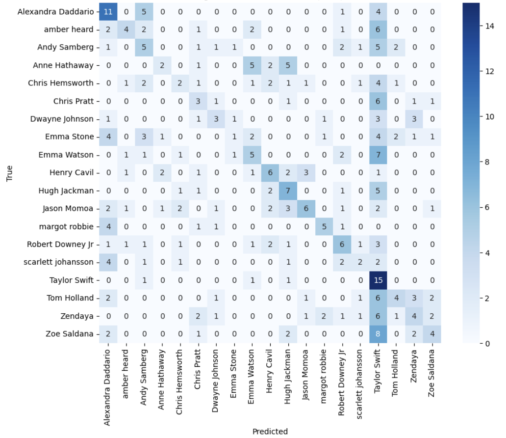
Figure 13: The confusion matrix of CNN model

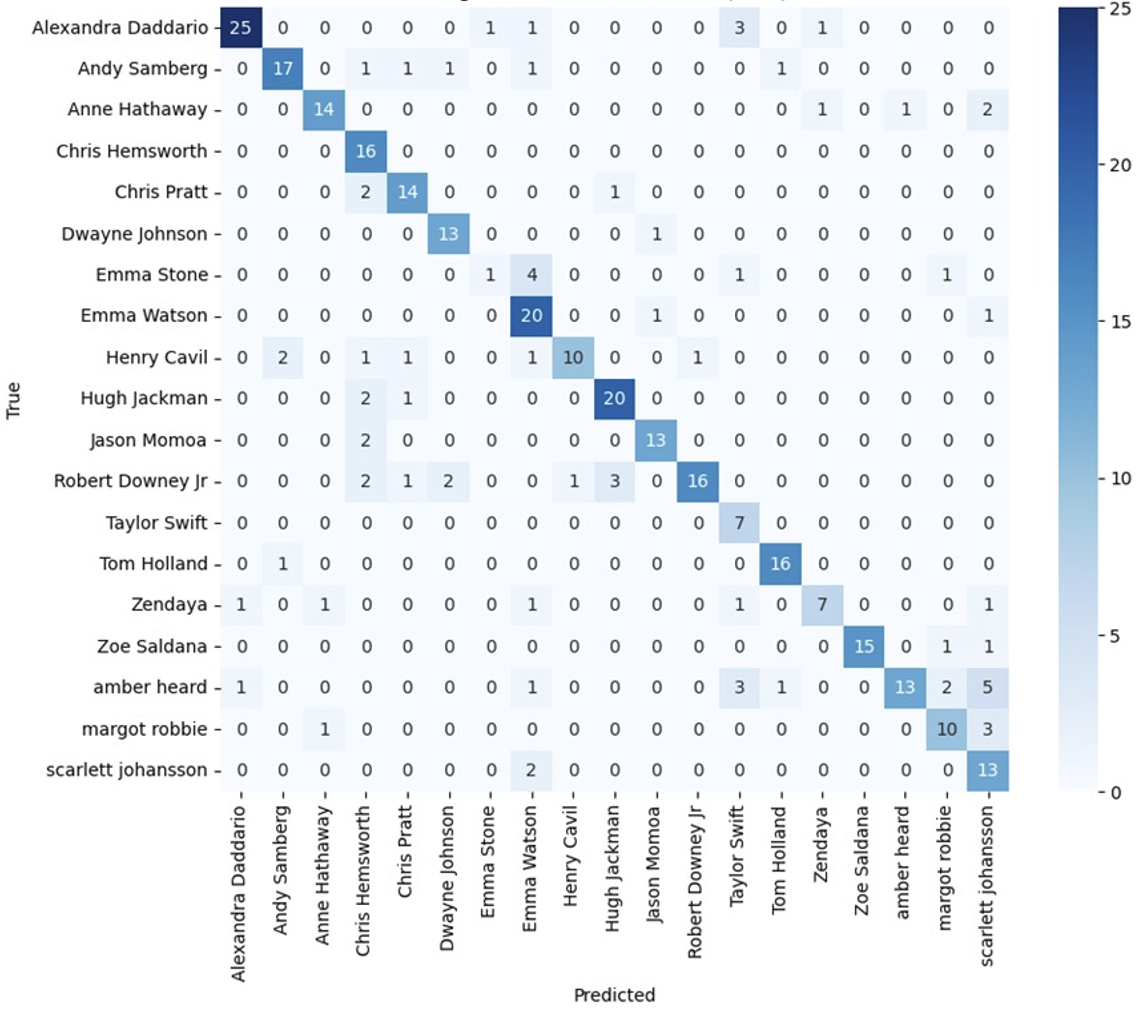
As shown in Figure 13, the high diagonal values indicate that most of the predictions are correct. It is worth noting that Emma Stone has a significantly lower diagonal value, which is consistent with the observation in Figure 11. In addition, we find a high misclassification between Emma Stone and Emma Watson, which may indicate that the model is having difficulty distinguishing between these two celebrities. This situation may be due to the failure of the model to capture the key features that distinguish these two celebrities.

3.2.3.3 Training, validation, and test accuracy

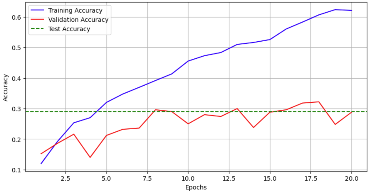
Figure 14: Training, Validation, and Test Accuracy (CNN)

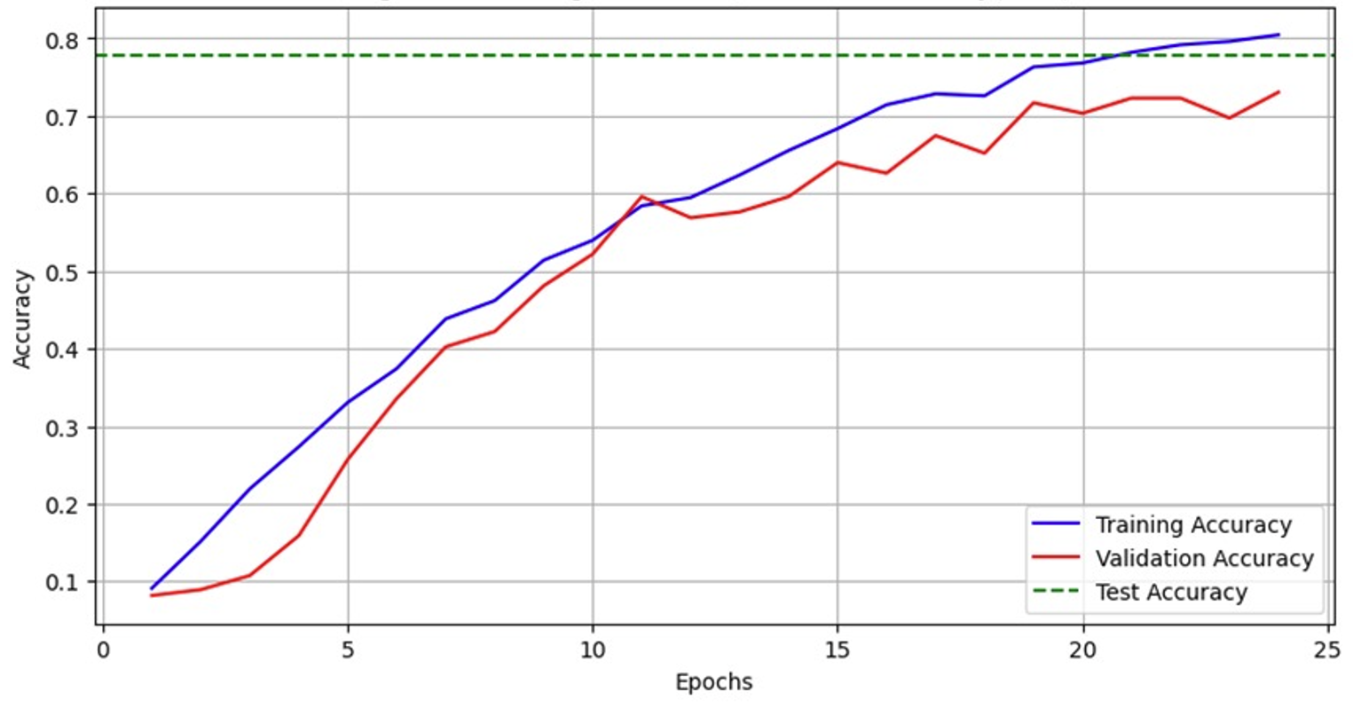
Figure 14 demonstrates the excellent performance of the CNN model on the training, validation, and test sets. The gradual increase in training and validation accuracy shows that the model is constantly learning and optimizing. The test accuracy is close to the validation accuracy. It reaches a value of almost 80%, indicating that the model has good generalization ability and can maintain high accuracy on new data.

3.3 Models Performance Comparison

Figure 15: Model comparison

As shown in figure 15, the ANN model demonstrated precision and recall at 0.33 and 0.29, respectively, with an F1 score and an accuracy of approximately 0.28. indicating struggles with false positives and negatives. The OpenCV-based model shows improvement, with all metrics around 0.43, suggesting fewer errors and a more balanced performance.

The CNN model significantly outperformed both the ANN and OpenCV models, with precision, recall, F1-score, and accuracy at levels of 0.81, 0.78, 0.78, and 0.78, respectively. 

Overall, the CNN model performed excellent on all metrics compared to the ANN and OpenCV models. It obtained the highest precision, recall, F1 score and accuracy scores, making it the most efficient and reliable model for this image recognition task.

3.4 Model Implementation

Following the evaluation of three models, the CNN model was selected as the most suitable implementation.

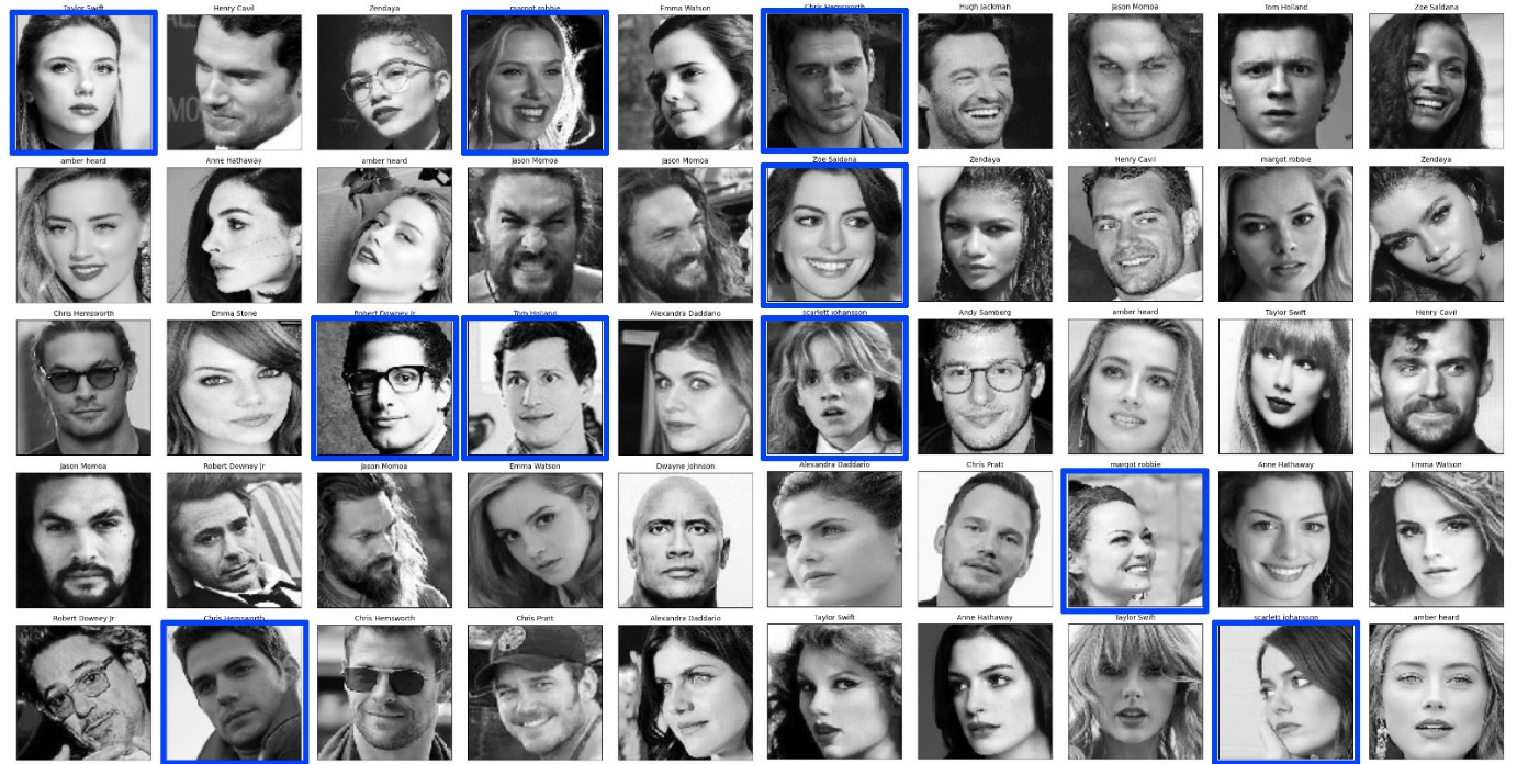
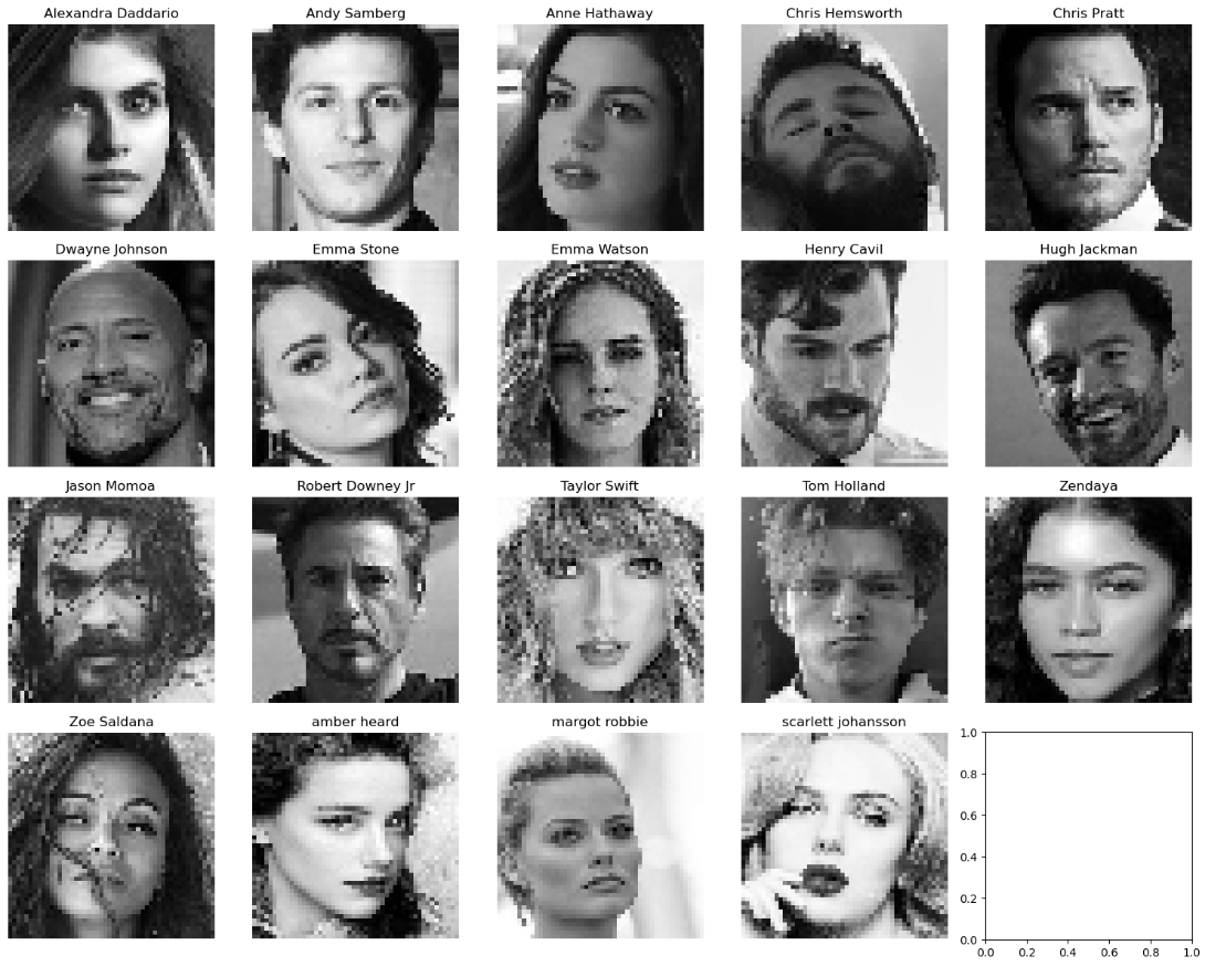
From the unlabelled dataset, we select the top 50 data for the prediction test. First, these 50 data are converted into images, and then the trained model is used for celebrity face recognition. The predicted name is displayed on top of the image. In this way, we have visualized the prediction results.

Figure 16: Convert data results to images for preview after prediction on unlabelled dataset

From the visualization of the results, we can see that out of these 50 characters, 10 people were incorrectly predicted. The accuracy of this prediction is therefore 80%. Additionally, we verified the predicted labels for the first 190 individuals in the unlabeled dataset, resulting in an accuracy of 77.4%.

In conclusion, the model demonstrated an approximate accuracy of 77% in practical applications. This indicates that the model has a high accuracy in practical applications.

4.Discussion

This study demonstrates the outstanding performance of CNN in image recognition tasks and reflects some valuable insights gained from different modelling approaches.

Firstly, this study has found that CNN perform best in facial recognition tasks. This advantage is primarily due to their strength in feature extraction, a crucial aspect of image classification tasks. Structurally, CNN contain convolutional layers that efficiently capture spatial hierarchies in images.

Secondly, from the performance of the three models, we found that Taylor Swift, Emma Stone, Zendaya and Dwayne Johnson performed worse. This could be because these celebrities had less data in the training set. The limited data makes it difficult for the model to learn their unique features efficiently, resulting in lower precision, recall and overall accuracy for these categories.

Therefore, it is concluded that the amount of training data plays a crucial role in the model's ability to classify images accurately.

Thirdly, the final CNN model's performance enhancements resulted from several optimizations. We employed data augmentation techniques to artificially increase the diversity of the training data, which helped the model generalize better. Additionally, we used freezing layers to retain the valuable low-level features learned from the MobileNetV2, which served as a feature extractor. These steps collectively led to a significant improvement in the CNN model's performance.

Finally, while CNN has demonstrated impressive performance in the face recognition task, we are optimistic about the potential for further enhancements.

To begin with, we can include a procedure to locate the face in the image before recognizing it. Once a face is detected, the system can automatically crop out the face region from the entire picture and analyze only this part. This step allows subsequent recognition algorithms to focus on the face region, thus significantly reducing the interference of background noise and improving recognition accuracy. 

Moreover, multiple different models can be integrated for learning, which can improve the system's robustness and accuracy. For example, the prediction results of multiple CNN models based on different architectures can be integrated to improve the overall recognition effect by voting or averaging. 

Additionally, the diversity and scale of datasets can be expanded. For instance, using web crawlers to automatically collect more images of celebrities from the Internet can result in more abundant training data, which can assist the model in learning and generalizing more effectively. 

Furthermore, by extending the application scenarios, we can move from binary classification to multi-classification tasks, identifying not only celebrities in images but also their specific activities or emotional states. This extension not only improves the system's utility but also enables it to be useful in a wider range of application scenarios.

5.Conclusion

This study aimed to achieve classification predictions for 19 specified celebrities based on input image data. We investigated three models, ANN, CNN, and OpenCV, respectively, and found that CNN performed best on all metrics. This result confirms the effectiveness of convolutional neural networks in face recognition tasks, especially when dealing with complex image data.